2D binary data classification using deep learning library Tensorflow – Keras

Keras is a high-level neural network library written in Python that can be run on TensorFlow or Theano. Keras has been developed with an emphasis on enabling rapid experimentation. It is important for good research to be able to go from idea to result with as little delay as possible.

Keras allows us to represent the desired network with relatively short code, such as only specifying the algorithms and parameters to be used in each layer, without having to implement the mathematical part behind DeepLearning from scratch.

This makes it possible to quickly try out the latest DeepLearning methods, which are flowing very fast in the research field and the latest implementations are being quickly adopted by companies.

Here the goal is to install, build model and execute training with simple 2D binary data set that has used in previous data classification.

The code is in below

#%%
import numpy as np
import matplotlib.pyplot as plt
from sklearn.datasets import make_circles
from sklearn.model_selection import train_test_split
from sklearn.metrics import classification_report
from keras.models import Sequential
from keras.layers import Dense
from keras.layers import Dropout

# データの準備
X, t = make_circles(n_samples=500, noise=0.2, factor=0.3)
t = t.astype('float')


plt.rcParams.update({'font.size': 18})
fig = plt.figure(figsize=(8, 8))
ax = fig.add_subplot(111, aspect='equal', xlim=(-2, 2), ylim=(-2, 2))
ax.plot(X[t ==  0, 0], X[t ==  0, 1], "rx")
ax.plot(X[t ==  1, 0], X[t ==  1, 1], "bx")


model = Sequential()
model.add(Dense(50, activation='relu', input_dim=2))
model.add(Dropout(0.5))
model.add(Dense(8, activation='tanh'))
model.add(Dense(1 , activation='sigmoid'))
model.compile(optimizer='adam',loss='binary_crossentropy',metrics=['accuracy'])

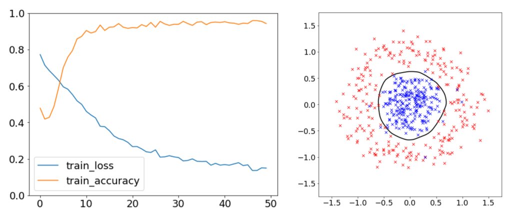
history = model.fit(X,t, epochs=50, batch_size=32)

fig = plt.figure(figsize=(8, 6))
ax = fig.add_subplot(111, ylim=(0, 1))
ax.plot(history.epoch, history.history["loss"], label="train_loss")
ax.plot(history.epoch, history.history["accuracy"], label="train_accuracy")
ax.legend()


XX, YY = np.meshgrid(np.linspace(-2, 2, 100), np.linspace(-2, 2, 100))
ZZ = model.predict(np.array([XX.ravel(), YY.ravel()]).T)
ZZ = ZZ.reshape(XX.shape)


fig = plt.figure(figsize=(8, 8))
ax = fig.add_subplot(111, aspect='equal', xlim=(-1.75, 1.75), ylim=(-1.75, 1.75))
ax.contour(XX, YY, ZZ, [0.5], colors='k', linewidths=2, origin='lower')
ax.plot(X[t ==  0, 0], X[t ==  0, 1], "rx")
ax.plot(X[t ==  1, 0], X[t ==  1, 1], "bx")

# %%