2D data clustering: Python simple Nonlinear SVM classification code

Now the classification was performed by nonlinear Support Vector Machine (SVM) – using Gaussian Kernel.
Goal here is to replace previous Linear SVM with Gaussian Kernel, then again compare the results with the one obtained from python scipy plugin – Sklern.

#%%
import numpy as np
from scipy.linalg import norm
import cvxopt
import cvxopt.solvers
from pylab import *

N = 500        # Data Amount
C = 20         # Slack variable
GAMMA = 5.0    # Parameter for Gaussian Kernel


# Gaussian Kernel
def gaussian_kernel(x, y):
    return np.exp(-norm(x-y)**2 / (2 * (GAMMA ** 2)))

# Calculate Descriminalt using only Support Vectors (since a[i] = 0 for non-support vectors)
def f(x, a, t, X, b):
    sum = 0.0
    for n in range(N):
        sum += a[n] * t[n] * gaussian_kernel(x, X[n])
    return sum + b


cls1 = []
cls2 = []

mean1 = [1,  4]
mean2 = [1, -3]
mean3 = [3, -2]
mean4 = [-2, 3]
cov = [[1.0,0.1], [0.5, 0.8]]

cls1.extend(np.random.multivariate_normal(mean1, cov, int(N/4)))
cls1.extend(np.random.multivariate_normal(mean3, cov, int(N/4)))
cls2.extend(np.random.multivariate_normal(mean2, cov, int(N/4)))
cls2.extend(np.random.multivariate_normal(mean4, cov, int(N/4)))

# Create Training Data Matrix X
X = vstack((cls1, cls2))

# Create Lavel t
t = np.array([1.0] * int(N/2) + [-1.0] * int(N/2))


# Calculate Lagrange Multiplier by using Quadratic Programming
K = np.zeros((N, N))
for i in range(N):
    for j in range(N):
        K[i, j] = t[i] * t[j] * gaussian_kernel(X[i], X[j])

Q = cvxopt.matrix(K)
p = cvxopt.matrix(-np.ones(N))
temp1 = np.diag([-1.0]*N)
temp2 = np.identity(N)
G = cvxopt.matrix(np.vstack((temp1, temp2)))
temp1 = np.zeros(N)
temp2 = np.ones(N) * C
h = cvxopt.matrix(np.hstack((temp1, temp2)))
A = cvxopt.matrix(t, (1,N))
b = cvxopt.matrix(0.0)
sol = cvxopt.solvers.qp(Q, p, G, h, A, b)
a = array(sol['x']).reshape(N)
#  print a

# Collect Support Vectors (Indexing)
S = []
M = []
for n in range(len(a)):
    if a[n] < 1e-5: continue
    S.append(n)
    if a[n] < 1e-5: continue
    if a[n] < C:
        M.append(n)


# Calculate bias parameter
sum = 0
for n in M:
    temp = 0
    for m in S:
        temp += a[m] * t[m] * gaussian_kernel(X[n], X[m])
    sum += (t[n] - temp)
b = sum / len(M)



# Show Training Data
plt.figure(figsize=(8, 6))
plt.rcParams.update({'font.size': 18})
x1, x2 = np.array(cls1).transpose()
plot(x1, x2, 'rx')

x1, x2 = np.array(cls2).transpose()
plot(x1, x2, 'bx')

# Show Support Vectors
for n in S:
    scatter(X[n,0], X[n,1], s=80, c='c', marker='o')

# Show Discriminant Boundary
X1, X2 = meshgrid(linspace(-6.3,6.3,100), linspace(-6.3,6.3,100))
w, h = X1.shape
X1.resize(X1.size)
X2.resize(X2.size)
Z = array([f(array([x1, x2]), a, t, X, b) for (x1, x2) in zip(X1, X2)])
X1.resize((w, h))
X2.resize((w, h))
Z.resize((w, h))
CS = contour(X1, X2, Z, [0.0], colors='g', linewidths=2, origin='lower')


# -----------------------------------------------------------------------------------------------------------
# Try same thing with sklearn!
from sklearn import svm

clf = svm.SVC(kernel='rbf', C=40, gamma=5)
X_train = np.vstack((cls1, cls2))
t = [-1] * int(N/2) + [1] * int(N/2)

clf.fit(X_train, t)

X1, X2 = meshgrid(linspace(-6,6,100), linspace(-6,6,100))
ZZ = clf.decision_function(np.c_[X1.ravel(), X2.ravel()])

ZZ.resize(X1.shape)
CS = contour(X1, X2, ZZ, [0.0], colors='k', linewidths=2, origin='lower')


xlim(-6, 7)
ylim(-7, 7)

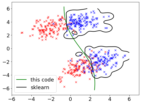
Green line shows the separation (counter line) from own code extended from the Linear SVM.
Black line shows the separation counter line from sklern – rbf that supposed to be closed to the Gaussian kernel.