Time series data fitting with Python polynomial regression
Polynomial regression is a problem of determining the complex relationship in observed data.
To be more specific, we can increase the coefficient of the regression equation to describe the nonlinearity as follows
f(x)=w0+w1x+w2x2+w3x3…
The question is how to determine the specific values of w0, w1, … of f(x)=w0+w1x+w2x2+… to obtain a curve close to the obtained data. In other words, our goal is to find w0, w1,… that minimize the square of the difference between f(x) and the measured value.
If we write it as a mathematical formula, it means to find w0, w1,… that minimize ∑i{yi-f(xi)}2.
If we set the derivative of ∑i{yi-f(xi)}2 by w0, w1,… to 0 respectively, we get the equation for |w| numbers. xi is arranged as X and yi is arranged as y. The equation can be written as follows
X’Xw’=X’y
Now, since the problem is to learn the weights of f(x), we can solve this using the least-squares method.
Goal here is to write own polynomial regression function that support nth order regression
import numpy as np
import matplotlib.pyplot as plt
# Design Matrix ==================================================
def basisFunctionVector (x, coefficient):
Phi = [x**i for i in range(coefficient+1)]
Phi = np.array(Phi).reshape(1, coefficient+1)
return Phi
## Obs values ------------------------------------------------------------------
X = np.array([0.10, 0.15, 0.20, 0.30, 0.40, 0.50, 0.58, 0.61, 0.65, 0.80, 0.85, 0.90])
Y = np.array([0.78, 0.80, 0.76, 0.69, 0.74, 0.71, 0.78, 0.92, 0.80, 0.85, 0.93, 0.98])
pred_X = np.arange(0, 1.1, 0.01)
# Order of coefficient
coefficient = 5
A = np.empty((0,coefficient+1), float)
for i in X:
A = np.vstack((A, basisFunctionVector (i, coefficient)))
#A'Ax = A'b, solve (A'A)x=A'b
ATA = np.dot(A.T, A)
Ab = np.dot(A.T, Y)
w = np.linalg.solve(ATA, Ab)
pred_Y = []
for i in pred_X:
temp = basisFunctionVector (i, coefficient)
pred_Y.append(np.dot(temp[0],w))
fig = plt.figure(figsize=(8, 6))
plt.plot(X, Y, 'ko')
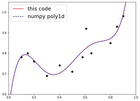
plt.plot(pred_X, pred_Y, 'r', label="this code")
plt.xlim(0.0, 1.0); plt.ylim(0.6, 1.05)
# -------------------------------------------
# Comparisons with numpy - polyfit
polynp = np.poly1d(np.polyfit(X, Y, coefficient))
plt.plot(pred_X, polynp(pred_X), 'b--', label="numpy poly1d")
plt.legend(loc="upper left", prop={'size': 14})
plt.xlim(0.0, 1.0); plt.ylim(0.6, 1.05)