2D data classification using Nonlinear SVM: explained with python code

SVM is a supervised machine learning algorithm that can be used for both classification and regression tasks, but in practice it is more commonly used for classification tasks.
It is a fast and reliable classification algorithm that can be expected to perform well with a small amount of data.

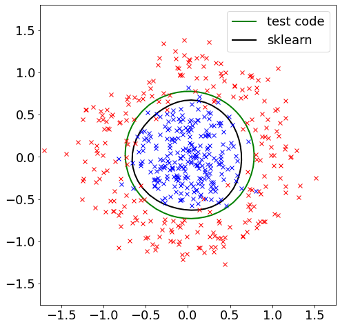
Now the classification was performed by nonlinear Support Vector Machine (SVM) – using Gaussian Kernel.
Goal here is to replace previous Linear SVM with Gaussian Kernel, then again compare the results with the one obtained from python scipy plugin – Sklern.

#%%
import numpy as np
import matplotlib.pyplot as plt
from sklearn.datasets import make_circles
from sklearn.model_selection import train_test_split
from sklearn.metrics import classification_report
from keras.models import Sequential
from keras.layers import Dense
from keras.layers import Dropout

# Data Preparation
X, t = make_circles(n_samples=500, noise=0.2, factor=0.3)
t = t.astype('float')


plt.rcParams.update({'font.size': 18})
fig = plt.figure(figsize=(8, 8))
ax = fig.add_subplot(111, aspect='equal', xlim=(-2, 2), ylim=(-2, 2))
ax.plot(X[t ==  0, 0], X[t ==  0, 1], "rx")
ax.plot(X[t ==  1, 0], X[t ==  1, 1], "bx")


model = Sequential()
model.add(Dense(50, activation='relu', input_dim=2))
model.add(Dropout(0.5))
model.add(Dense(8, activation='tanh'))
model.add(Dense(1 , activation='sigmoid'))
model.compile(optimizer='adam',loss='binary_crossentropy',metrics=['accuracy'])

history = model.fit(X,t, epochs=50, batch_size=32)

fig = plt.figure(figsize=(8, 6))
ax = fig.add_subplot(111, ylim=(0, 1))
ax.plot(history.epoch, history.history["loss"], label="train_loss")
ax.plot(history.epoch, history.history["accuracy"], label="train_accuracy")
ax.legend()


#print(classification_report(t, model.predict(X)))

XX, YY = np.meshgrid(np.linspace(-2, 2, 100), np.linspace(-2, 2, 100))
ZZ = model.predict(np.array([XX.ravel(), YY.ravel()]).T)
ZZ = ZZ.reshape(XX.shape)


fig = plt.figure(figsize=(8, 8))
ax = fig.add_subplot(111, aspect='equal', xlim=(-1.75, 1.75), ylim=(-1.75, 1.75))
ax.contour(XX, YY, ZZ, [0.5], colors='k', linewidths=2, origin='lower')
ax.plot(X[t ==  0, 0], X[t ==  0, 1], "rx")
ax.plot(X[t ==  1, 0], X[t ==  1, 1], "bx")
a = 1
# %%