2D multi-class categorical data classification using Tensorflow

The case where there are not only “0” and “1” but also “2”, “3” to “9” and many other classification categories (=classes) is called multi-class classification. This is a case where there are many classification categories (=classes), not only “0” and “1” but also “2”, “3” to “9”. In this case, “0” to “9 are called class indexes (some libraries refer to them as sparse labels). .

Class indexes are mainly assigned to categorical variables (categorical variables). For example, if you have categorical variables like “cat” “tiger” and “lion”, then you can assign category as follows: “cat=0,” “tiger=1,” “lion=2.
This kind of assignment is called categorical variable encoding, and the method of encoding into class indexes in particular is called integer encoding.

When it comes to the numerical encoding, one of the most famous technique is “one-hot encoding”. This is a method of encoding where variables (mathematically “vectors”, programming-wise “arrays”) are prepared for the number of categories, and only one of them is set to 1, while the others are set to 0. For example, if there are 10 categories (e.g., cat, tiger, ……, puma) and the corresponding category variable is the class index (e.g., cat = 0, tiger = 1, ~, puma = 9), prepare 10 variables, e.g., the 10th one (= class index is 9) so that only that variable is 1 and the others are 0. In other words, class index 9 is described as

“0, 0, 0, 0, 0, 0, 0, 0, 0, 0, 1”

While one-hot encoding is intuitive and convenient for multi-class classification, it has the disadvantage of requiring special encoding as described above.

Whether we use class indexes or one-hot multiple variables, unlike the binary classification described above, there cannot be only one neuron in the output layer. For example, if there are more than three variables such as “cat”, “tiger”, and “lion” (……), the output layer must also have more than three neurons corresponding to each of them.

As in the case of binary classification, it is easier to express the values output by the neurons in the output layer as 100% probability values. For example

Example of output values 1: “Cat = 3.2”, “Tiger = 1.2”, “Lion = 0.3”.
Example of output values 2: “Cat = 10.2”, “Tiger = 5.2”, “Lion = 0.6
Rather than outputting the predicted result values of

Example output value 1: “Cat = 68.1%”, “Tiger = 25.5%”, “Lion = 6.4%”
Example output value 2: “Cat = 63.7%, Tiger = 32.5%, Lion = 3.8%”
It would be easier to understand and compare (e.g., in Example 1 and Example 2) if the values were described as 100% probability values.

The activation function that brings the total number of multiclasses to 100% is the Softmax function.

Even when a softmax function is used as the activation function for multiclass classification, the loss function used in the set is basically fixed. Specifically, it is the Categorical Cross Entropy for multi-class classification. The calculation method is different from the one for binary classification, but in short, the basic idea is to use cross entropy for classification.

Below code perform categorical data classification with relu and softmax activation with Keras package.

#%%

import numpy as np
import matplotlib.pyplot as plt

from sklearn.model_selection import train_test_split
from sklearn.metrics import classification_report
from keras.models import Sequential
from keras.layers import Dense
from keras.layers import Dropout
from tensorflow.keras.utils import to_categorical
#
N = 300 # number of points per class
D = 2 # dimensionality
K = 6 # number of classes
X = np.zeros((N*K,D)) 
y = np.zeros(N*K) 
for j in range(K):
    ix = range(N*j,N*(j+1))
    r = np.linspace(0.0,1,N) 
    t = np.linspace(j*4,(j+1)*4,N) + np.random.randn(N)*0.2 
    X[ix] = np.c_[r*np.sin(t), r*np.cos(t)]
    y[ix] = j


model = Sequential()
model.add(Dense(200, activation='relu', input_dim=D, kernel_initializer='he_uniform'))
model.add(Dense(50, activation='relu', input_dim=D, kernel_initializer='he_uniform'))
model.add(Dense(6, activation='softmax'))
model.compile(optimizer='adam',loss='categorical_crossentropy',metrics=['accuracy'])
t = to_categorical(y)

#
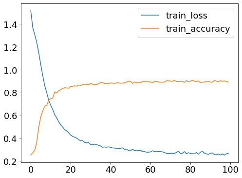
history = model.fit(X,t, epochs=100)

plt.rcParams.update({'font.size': 18})
fig = plt.figure(figsize=(8, 6))
ax = fig.add_subplot(111)
ax.plot(history.epoch, history.history["loss"], label="train_loss")
ax.plot(history.epoch, history.history["accuracy"], label="train_accuracy")
ax.legend()
plt.show()



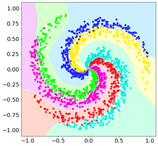
XX, YY = np.meshgrid(np.linspace(-1.1, 1.1, 200), np.linspace(-1.1, 1.1, 200))
ZZ = model.predict(np.array([XX.ravel(), YY.ravel()]).T)
ZZ = np.argmax(ZZ, axis=1)
ZZ = ZZ.reshape(XX.shape)


fig = plt.figure(figsize=(8, 8))
ax = fig.add_subplot(111, aspect='equal', xlim=(-1.1, 1.1), ylim=(-1.1, 1.1))
ax.scatter(X[:, 0], X[:, 1], c=y, s=30, cmap=plt.cm.gist_rainbow)
ax.contourf(XX, YY, ZZ, cmap=plt.cm.gist_rainbow, alpha=0.2)
ax.contour(XX, YY, ZZ, colors='w', linewidths=0.4)

# %%