Determine optimal number of regression coefficient by AIC

In a previous post, it was demonstrated that using larger number of polynomial regression coefficient increases the accuracy of the data fitting. In practical case however, larger number of polynomial coefficient will overfit the data, capturing unnecessary noise from data and/or reduce the quality of the cross-validation results.

Goal here is to use Akaike Information Criteria (AIC) to estimate trade-off between best fit of the model and model complexity, demonstrate using 1D regression example.

AIC = -2(log-likelihood) + 2K

import numpy as np
import matplotlib.pyplot as plt

# Design Matrix ==============================================
def basisFunctionVector (x, feature):
    Phi = [x**i  for i in range(feature+1)]
    Phi = np.array(Phi).reshape(1, feature+1)
    return Phi
# ============================================================



## Set Parameters for AIC -------------------------------------
MaxAIC = 20          # maximum polynomial
LL   = []            # log-likelihood
AIC  = []            # Calculated AIC          


fig = plt.figure(figsize=(15,10))
for feature in range(MaxAIC):

    ## Set Input parameters ----------------------------------------------------
    N = 20                              # number of data
    X = np.linspace(0.05, 0.95, N)         # x parameter
    Y = np.array([0.85, 0.78, 0.70, 0.76, 0.77, 0.69, 0.80, 0.74, 0.76, 0.76,
                  0.81, 0.79, 0.80, 0.84, 0.88, 0.89, 0.86, 0.93, 0.97, 0.98])
    pred_X = np.arange(0, 1, 0.01)
    ## -------------------------------------------------------------------------


    A = np.empty((0,feature+1), float)
    for x in X:
        A = np.vstack((A, basisFunctionVector (x, feature))) 

    ## Compute weight (Maximum likelihood) ------------------------------------
    w = np.linalg.solve(np.dot(A.T, A), np.dot(A.T, Y))


    ## Compute SigmaSq of Gaussian Noise (Maximum likelihood) -----------------
    SigmaSq = 0
    for i in range(len(X)):
        SigmaSq += (Y[i] - np.dot(A[i],w))**2
    SigmaSq = SigmaSq / len(X)


    ## Compute log-likelihood / AIC (Gaussian Noise Case) ----------------------
    LL.append(-0.5*N*np.log(2*np.pi*SigmaSq)-N/2)       
    AIC.append(-2*LL[feature]+2*(len(w)+1))

    plt.subplot(4, MaxAIC/4, feature+1)

    plt.xlim(0.0, 1.0)
    plt.ylim(0.6, 1.05)
    plt.plot(X, Y, 'ko')    # Obs data   
    pred_Y = []
    for x in pred_X:
        temp = basisFunctionVector (x, feature)
        pred_Y.append(np.dot(temp[0],w))
    plt.plot(pred_X, pred_Y, 'r')   
    plt.title("Polynomial order = " + str(feature)); 

plt.subplots_adjust(hspace = 0.3)
plt.show()

fig = plt.figure(figsize=(11,5))
plt.subplot(1, 2, 1)
plt.rcParams.update({'font.size': 18})
xlist = np.arange(1, MaxAIC+1, 1)
plt.plot(xlist, LL, 'bo-')
plt.xlabel('Order of Polynomical')
plt.title("Log-likelihood"); 

plt.subplot(1, 2, 2)
plt.rcParams.update({'font.size': 18})
plt.plot(xlist, AIC, 'bo-')
plt.xlabel('Order of Polynomical')
plt.title("AIC"); 
plt.show()

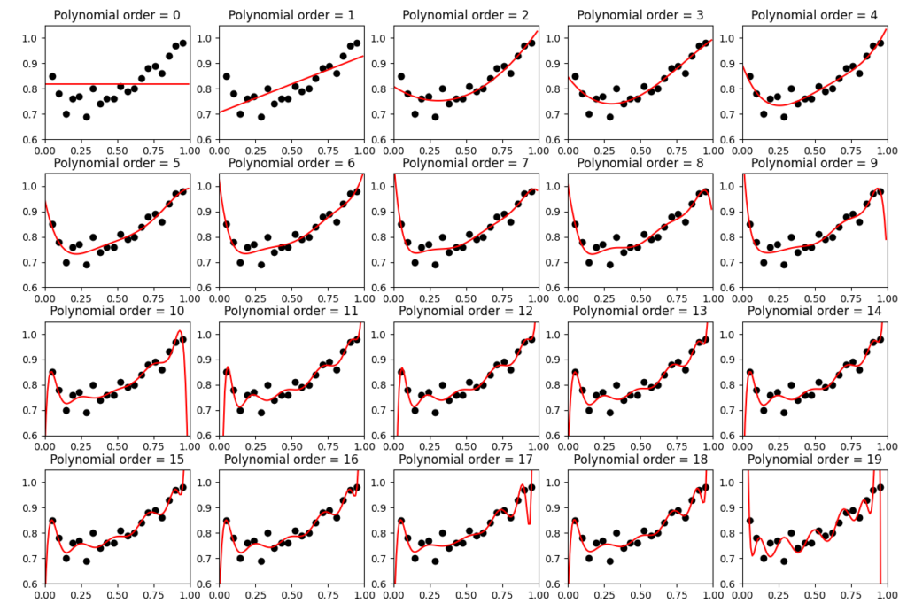
Below shows result of polynomial regression by changing number of coefficient.

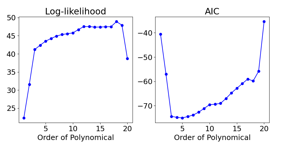
Below shows estimate of AIC and likelihood in log scale, used to estimate equation
AIC = -2(log-likelihood) + 2K.

As expected, Log-likelihood kept increasing as the number of coefficient increases. The value increased when the number of coefficient gets higher than 19, potentially increased the misfit from few data points.

For AI value, we can find that value decreases till number of coefficient by 5, while start increasing with more coefficient added in regression equation.

Based on the results, optimal number of coefficient is 5 by estimate of AIC, and 3 would be the practical best choice as the improvement of fitting (increase of Log-likelihood) is small between 3~5.