Python template for scientific histogram plot

A histogram is a bar graph that shows the number of data belonging to each section as a height, with the width of the section having a boundary value according to the numerical value of the data, and is used to estimate the shape of the population distribution behind the data, as well as its center position and variability.

It is easy to create a histogram using software such as Excel. However, creating nice histogram plot for scientific paper and presentation is always pain as many features need to be customize manually.

Goal here is to provides basic histogram plot with cosmetic customization.

Creating graphs in Python can be done easily by using useful libraries such as matplotlib. If you do not have matplotlib installed on your library, you can start by typing the following command in a terminal.

pip install matplotlib

Recently, the Anaconda package, a development environment that includes libraries for data analysis is frequently used instead of Python directly. If you have Anaconda installed, matplotlib is also installed at the same time, so there is no need to install matplotlib.

To use matplotlib, you need to write a description to import it into your program.

import matplotlib.pyplot as plt

This imports the matplotlib.pyplot module with the name plt.

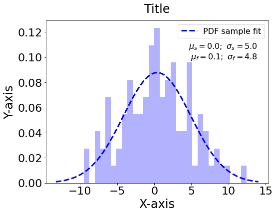
Below code plot gaussian sample generated by numpy random function, then used matplotlib hist function with additional cosmetics to alter the color, add pdf and statistics in a plot.

import numpy as np
from matplotlib import pyplot as plt
from scipy.stats import norm


#------------------------------------------------------------
#- Template function to generate scientific histogram plot

def customHistPlot(sample,titleP='Title',titleX='X-axis',titleY='Y-axis'):
    # Plot the sampled data
    fig, ax = plt.subplots(figsize=(8, 6))
    ax.hist(sample, 30, histtype='stepfilled', density=True, fc='#0000FF', alpha=.3)

    sample_mu = np.mean(sample)
    sample_std = np.std(sample, ddof=1)
    pdf_range = [sample_mu - sample_std*3,sample_mu + sample_std*3]
    x = np.linspace(pdf_range[0],pdf_range[1], 1000)
    ax.plot(x, norm.pdf(x, sample_mu, sample_std), '--b', label='PDF sample fit',linewidth=3.0)

    ax.legend(loc=0, fontsize=16)

    ax.set_title(titleP,fontsize=24,pad=15)
    ax.set_xlabel(titleX,fontsize=24)
    ax.set_ylabel(titleY,fontsize=24)
    for label in ax.xaxis.get_ticklabels():label.set_fontsize(22)
    for label in ax.yaxis.get_ticklabels():label.set_fontsize(22)

    ax.text(0.95, 0.87, ("$\mu_s=0.0;\ \sigma_s=5.0$\n"
                        "$\mu_f=0.1;\ \sigma_f=4.8$\n"),
                transform=ax.transAxes, ha='right', va='top', fontsize=16)
    plt.show()

#----------------------------------------------------
#- Test


input_mu = 0
input_std = 5
num_samples = 100
sample = np.random.normal(input_mu, input_std, num_samples)

customHistPlot(sample)


# %%