Time series data fitting with Ordinary Kriging regression

Kriging is a method often used in geostatistical science, and is called a Gaussian process in the popular field of machine learning.

Kriging is one of the spatial interpolation methods originally proposed by D.G. Krige. It is a method for spatial interpolation that uses the spatial correlation structure that data from observation points that are close in distance have a large similarity.

Algorithm is to interpolate between measured data point via unbiased minimum variance estimation, as described in Wikipedia.

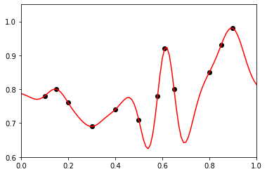
Below code shows dimple implementation of ordinary kriging regression and with application for 1D time series data fitting using gauss variogram function.

#%%

import numpy as np
import matplotlib.pyplot as plt
from numpy import linalg


def Test_Okriging(x,Obsp,xx,nget,sill,rnge):

    nobs = len(Obsp)

    A  = np.ones((nobs+1,nobs+1)) # +1 for lagrange multiplier
    b  = np.ones((nobs+1,1))
    Cd = np.ones((nobs+1,nobs+1))

    b[nobs]= 1   # 1 = lagrange multiple

    # Variogram_Generation(Cd,A,Obsp,pos,nget,sill,rnge)
    #------------------------------------------------
    #  Covariance Generation by Data-Data Distance
    for i in range(nobs):
        for j in range(i, nobs) :
            Cd[i][j] = np.linalg.norm(x[i]-x[j])


    #------------------------------------------------
    # Variogram: Spherical/Gaussian Method
    for i in range(nobs) :
        for j in range(i, nobs) :
            A[i][j] = A[j][i] = nget + sill*np.exp(-3*Cd[i][j]**2/(rnge**2))


    #---------initialize values--------

    vvval = np.ones((int(len(xx))))

    for i in range(len(xx)):

        for k in range(nobs) :

            distance = np.linalg.norm(xx[i]-x[k])

            b[k] = nget + sill*np.exp(-3*distance**2/(rnge**2))
 
        Weit  = linalg.solve(A,b)

        OKest = np.sum([Weit[j]*Obsp[j] for j in range(0, nobs)])

        vvval[i] = OKest

    #--------- Return! ---------
    return vvval




#------------------------------------------
# Observed Data
#------------------------------------------

X = np.array([0.10, 0.15, 0.20, 0.30, 0.40, 0.50, 0.58, 0.61, 0.65, 0.80, 0.85, 0.90])
Y = np.array([0.78, 0.80, 0.76, 0.69, 0.74, 0.71, 0.78, 0.92, 0.80, 0.85, 0.93, 0.98])
pred_X = np.arange(0, 1.1, 0.01)    
 
#------------------------------------------
# Ordinary Kriging Estimation
#------------------------------------------

pred_Y = Test_Okriging(X,Y,pred_X,0.0,0.1,0.12)

plt.plot(X, Y, 'ko') 
plt.plot(pred_X, pred_Y, color = 'red')
plt.xlim(0.0, 1.0); plt.ylim(0.6, 1.05)
plt.show()

# %%