Time series data fitting with SciPy Gaussian Process Regression

In general, the prediction accuracy of machine learning is high in areas where there is a lot of data, and low in areas where there is no data. High prediction accuracy (reliability of prediction values) is an important factor for machine learning models, but general regression analysis methods (Partial Least Squares, Support Vector Regression, etc.) cannot evaluate the prediction reliability.

One solution to this problem is the Gaussian Process.

The Gaussian Process (GP) is a machine learning method that mainly performs regression analysis. One of its main features is that it outputs the distribution of the predicted values of the target variable y for the input of the explanatory variable X as a normal distribution.

f(X)=N(μ,σ2)

The standard deviation σ of the output normal distribution represents the “uncertainty” of the value of the target variable y. Data with a small standard deviation σ are more uncertain. Data with a small standard deviation σ can be judged to have a small uncertainty (high predictive reliability), while data with a large standard deviation σ can be judged to have a large uncertainty (low predictive reliability), allowing us to perform regression analysis considering the predicted value + the reliability of the predicted value.

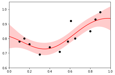
import numpy as np
import matplotlib.pyplot as plt
from sklearn import gaussian_process
from sklearn.gaussian_process.kernels import RBF,WhiteKernel, ConstantKernel

#------------------------------------------
# Observed Data
#------------------------------------------

X = np.array([0.10, 0.15, 0.20, 0.30, 0.40, 0.50, 0.58, 0.61, 0.65, 0.80, 0.85, 0.90])
Y = np.array([0.78, 0.80, 0.76, 0.69, 0.74, 0.71, 0.78, 0.92, 0.80, 0.85, 0.93, 0.98])
pred_X = np.arange(0, 1.1, 0.01)    

X = X.reshape(-1,1)
pred_X = pred_X.reshape(-1,1)


#------------------------------------------
# Ordinary Kriging Estimation
#------------------------------------------

regressor = gaussian_process.GaussianProcessRegressor(kernel=ConstantKernel() * RBF(), normalize_y=True, alpha=0.2)
pred_Y, pred_Std = regressor.fit(X, Y).predict(pred_X, return_std=True)


plt.plot(X, Y, 'ko') 
plt.plot(pred_X, pred_Y, color = 'red')
plt.fill_between(np.arange(0, 1.1, 0.01) , pred_Y - 2 * pred_Std, pred_Y + 2 * pred_Std, alpha=0.2, facecolor='red',)
plt.xlim(0.0, 1.0); plt.ylim(0.6, 1.05)
plt.show()


# %%

The input kernel function is a key to generate reasonable regression model.

The Constant Kernel is the constant kernel, the RBF Kernel is the Radius Based Function kernel (or Gaussian kernel), and the White Kernel is the kernel function for the magnitude of the noise in the objective variable, which is useful when the dataset contains noise (although not relevant in this case). Note that when introducing the White Kernel, the argument alpha of GaussianProcessRegressor should be set to 0.

Running the fit function of GaussianProcessRegressor will train the GP model. If not specified otherwise, the parameters of the kernel function will be optimized to maximize the likelihood for the model building data.